Model-based / Model-free RL
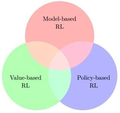
Everybody knows reinforcement learning is one of a machine learning methods aiming to make agent explore and find the optimal policy through interactions with environment and maximize cumulative reward. Before starting this passage, we have to understand what is model-free and what is model-based?

Monte-Carlo (MC)
Overview
The Monte Carlo algorithm is a broad class of computational algorithms that rely on repeated random sampling to obtain numerical results. The core idea is to use randomness to solve problems that might be deterministic in principle. The key concepts of MC are: random sampling, estimation by taking the average of outcomes from random samples, applicability of high-dimensional spaces. It can be used in simulations, optimization, numerical integration, financial anticipation and statistical physics. Advantages and disadvantages of MC are shown in the table below.
| Monte Carlo | Advantages | Disadvantages |
|---|---|---|
| 1 | Simple to implement | Can be computationally intensive |
| 2 | Flexible and can handle a wide range of problems | Convergence can be slow |
| 3 | Suitable for high-dimensional integrals | Results are probabilistic, not deterministic |
Here is a classic example of MC application: Estimate the value of $π$.
1 | import random |
The result is π: 3.13544.
Assuming we have a state sequence under a policy π:
$$
[S_1,A_1,R_1,S_2,A_2,R_2,S_3,A_3,R_3,…,S_T,A_T,R_T]\tag{1}
$$
In MDP, the value function is:
$$
v_π(s)=E_π[G_t|S_t=s]G_t=R_{t+1}+γR_{t+2}+…+γ^{T−t−1}R_Tv_π(s)≈average(G_t)\tag{2}
$$
However, the average consumes so many storage. A better method is obtaining average value in iterations:
$$
μt=\frac 1 t ∑j=\frac 1 t x_j=\frac 1 t (x_t+\sum_{j=1}^{t−1}x_j)=μ_{t−1}+\frac 1 t (x_t−μ_{t−1})\tag{3}
$$
Q Learning: the first step of model-free RL
Algorithm
Q learning is a value-based RL algorithm. Thus, Q value is the fundamental variable in this algorithm, and this is the reason why this algorithm called “Q Learning”. Assuming we already know what is agent, what is environment, what are the states, the actions have to be discrete and the reward function, let us cut to the point and introduce the learning method of agent in Q Learning.
$$
Q(s,a)\leftarrow Q(s,a)+α(r+γmax_{a^′}Q(s^′,a^′)−Q(s,a))\tag{4}
$$
Equation above is the update method of Q value. α is learning rate (basically learning rate defines the pace of updating), γ is discount factor. $Q(s,a)$ is the action value of current state; $Q(s^′,a^′)$ is the action value of next state; $max_{a^′}Q(s^′,a^′)$ means choosing the maximum $Q(s^′,a^′)$ among all the possible actions.
The Q learning is quite similar to value iteration. We are going to explain the differences between Q learning and value iteration in detail through a simple implementation.
Implementation
Environment
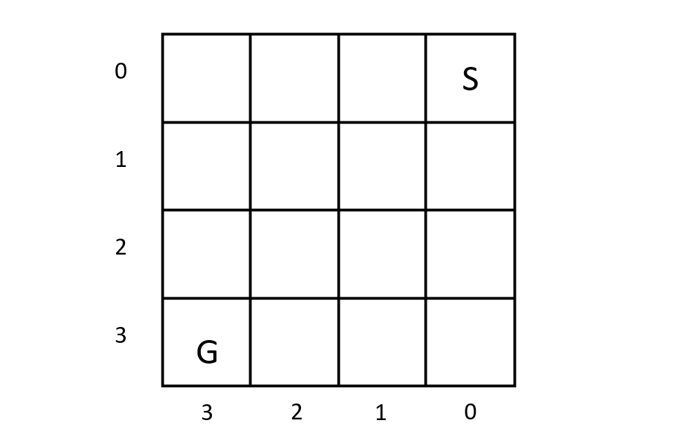
The environment is a 4x4 grid. Our target is to train the agent and let it successfully moves from (0, 0) to (3,3).

1 | grid_size = 4 |
Hyperparameters
$ϵ$ means the agent have probability equals to ϵ choosing a random action and $(1-ϵ)$ probability choosing the optimal action.
1 | alpha =0.1 #learning rate |
State(s) and action(s)
The state is just all the points in the 4x4 girds. We create two functions for action selection and transition to next state.
In function get_next_state, the current coordinates based on the action:
- If the action is
'up'andxis greater than 0, it moves up by decrementingxby 1. - If the action is
'down'andxis less thangrid_size - 1, it moves down by incrementingxby 1. - If the action is
'left'andyis greater than 0, it moves left by decrementingyby 1. - If the action is
'right'andyis less thangrid_size - 1, it moves right by incrementingyby 1.
1 | def get_next_state(state, action): |
Reward function
Agent will get reward = 100 if arriving at (3, 3), otherwise -1.
1 | def get_reward(state): |
Q value function
This part is the fundamental training loop of algorithm. while state != goal_state means continues iterations until the goal state is reached; action_index = choose_action(state) means select an action index based on policy which not shown; action = actions[action_index]is to convert the action index to an actual action; next_state = get_next_state(state, action) is used to determine the next state based on the current state and action; finally,reward = get_reward(next_state)can calculate the reward for transitioning to the next state.
Then, we store Q value under current (s, a) pair in Q table, computes the maximum Q value for next state and updates Q value for current $(s,a)$ pair using Q learning update rule.
Since we have the maximum Q value of each state stored in Q table, we can try to compute the optimal policy and turn it into the form of path.
1 | for episodeinrange(num_episodes): |
Results
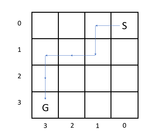
The path after training is shown in the figure.

Sarsa: An on-policy RL algorithm
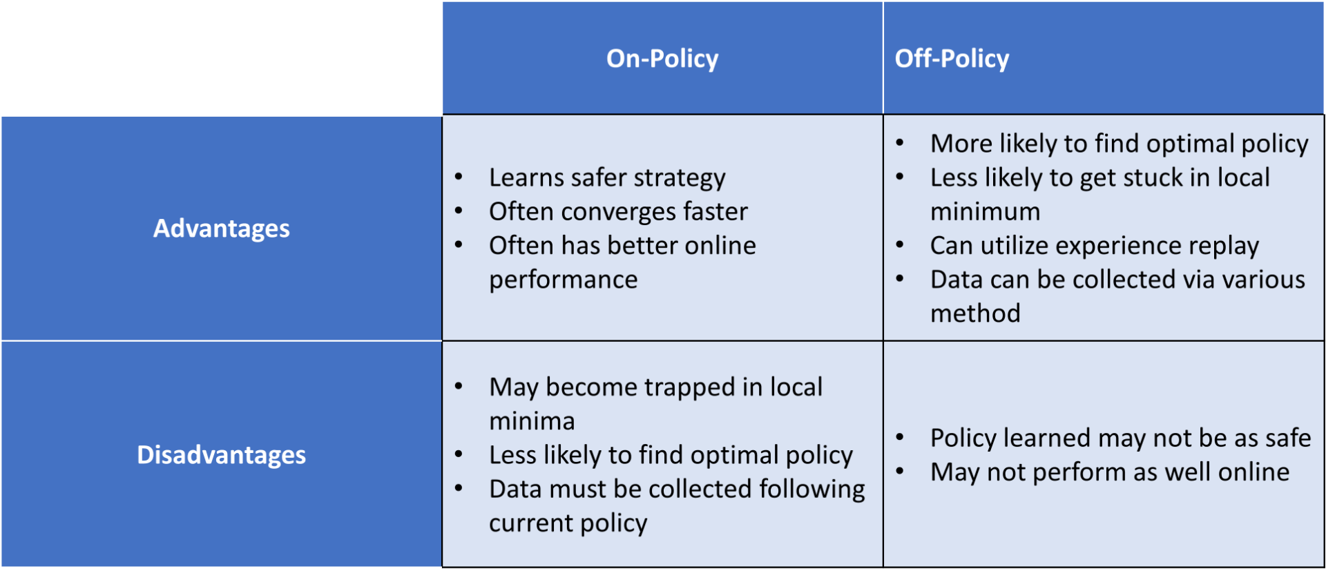
Difference between on-policy & off-policy
In reinforcement learning, two different policies are also used for active agents: a behavior policy and a target policy. A behavior policy is used to decide actions in a given state (what behavior the agent is currently using to interact with its environment), while a target policy is used to learn about desired actions and what rewards are received (the ideal policy the agent seeks to use to interact with its environment).
If an algorithm’s behavior policy matches its target policy, this means it is an on-policy algorithm. If these policies in an algorithm don’t match, then it is an off-policy algorithm.

Sarsa operates by choosing an action following the current epsilon-greedy policy and updates its Q values accordingly. On-policy algorithms like Sarsa select random actions where non-greedy actions have some probability of being selected, providing a balance between exploitation and exploration techniques. Since Sarsa Q values are generally learned using the same epsilon-greedy policy for behavior and target, it classifies as on-policy.
Q learning, unlike Sarsa, tends to choose the greedy action in sequence. A greedy action is one that gives the maximum Q value for the state, that is, it follows an optimal policy. Off-policy algorithms like Q learning learn a target policy regardless of what actions are selected from exploration. Since Q learning uses greedy actions, and can evaluate one behavior policy while following a separate target policy, it classifies as off-policy.
Algorithm
SARSA, unlike Q learning, is an on-policy algorithm, which means it updates the policy based on the actions taken. Quite like policy iteration. But in Sarsa, the update of policy will not be as “hard” as policy iteration since we have the influence of learning rate $α$.
Still, the algorithm keeps updating Q value. One thing different is agent of Sarsa already come up with which action to choose and predict next state and next action. That is why the algorithm called SARSA - State, Action, Reward, State, Action.
Implementation
code
1 | import numpy as np |
Result
1 | State: (0, 0) |